SpectralClustering
Spectral clustering uses networks of neighbors rather than proximity to some centroid to partition data. This means it has the ability to to cluster concentric circles as in the “bull’s eye” example, but practially speaking the benefit is that spectral clustering doesn’t constrain cluster shape to being convex. I think that it’s a more natural treatment for a lot of datasets and often results in improved results relative to more commonly used methods. Plus it involves a pretty elegant matrix decomposition step.
Spectral refers to the fact that it uses eigenvectors of a network
proximity matrix. That’s the most surprising part of the technique to
me. If your data can be coerced to a properly normalized similarity
matrix, which can also be though of as a network connectivity matrix, It
turns out that the eigenvectors corresponding to the lowest non-zero
eigenvalues can be used to identify optimal cut-points in the network.
If your data are not already in network form, they can be made into a
network by converting them a proximity matrix. This is where the second
great feature of spectral clustering comes in. Non-linear distance
kernels can be be used to create the proximity network giving us a
tuneable non-linearity similar to support vector machines.
Drawbacks to spectral clustering are (1) in most cases it requires you to tune at least one new hyperparameter for the distance kernel (eg sigma for a gaussian kernel) and (2) it’s not a great fit out-of-the box for big datasets. The proximity network can get pretty big and the matrix decomposition can also be a challenge.
Example
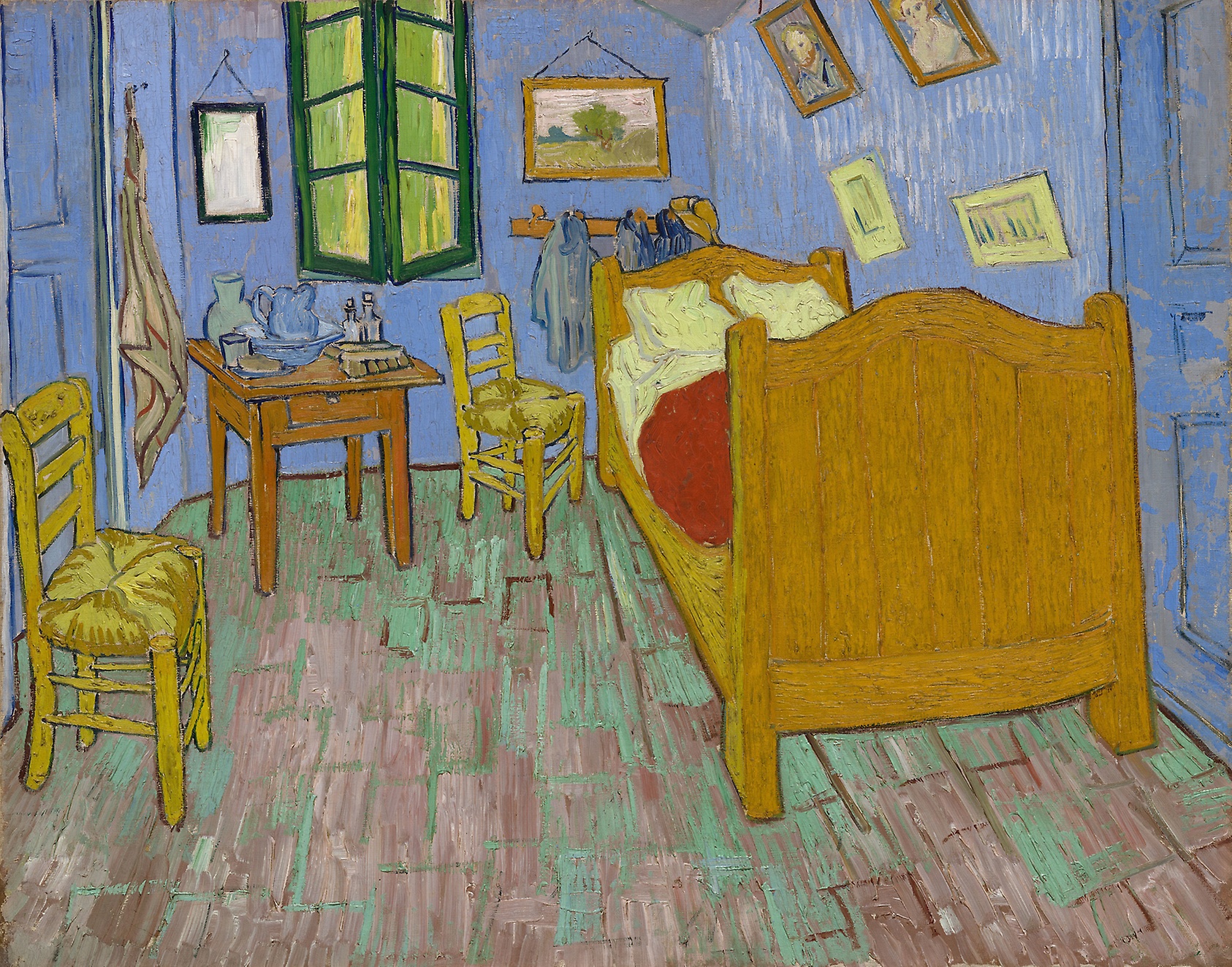
I’m clustering pixels in the famous painting “The Bedroom” to demonstrate the elements of spectral clustering. I will reduce the painting to just a handful of colors. I hope that this example will be an intuitive explanation of the technique: more detailed treatment of spectral clustering can be found here and here. I’m just trying to elaborate on what I like about this technique and make some useful visualizations.
Raw Data
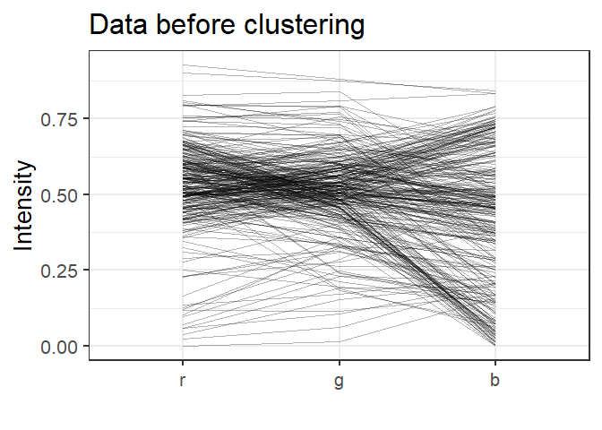
Red, green and blue intensities were plotted for a subset of 300 data points. Several clusters are already apparent in the data. Prior to defining clusters, though, we will transform the data into a similarity matrix.
Similarity Matrix, Eigenvectors and Clustering
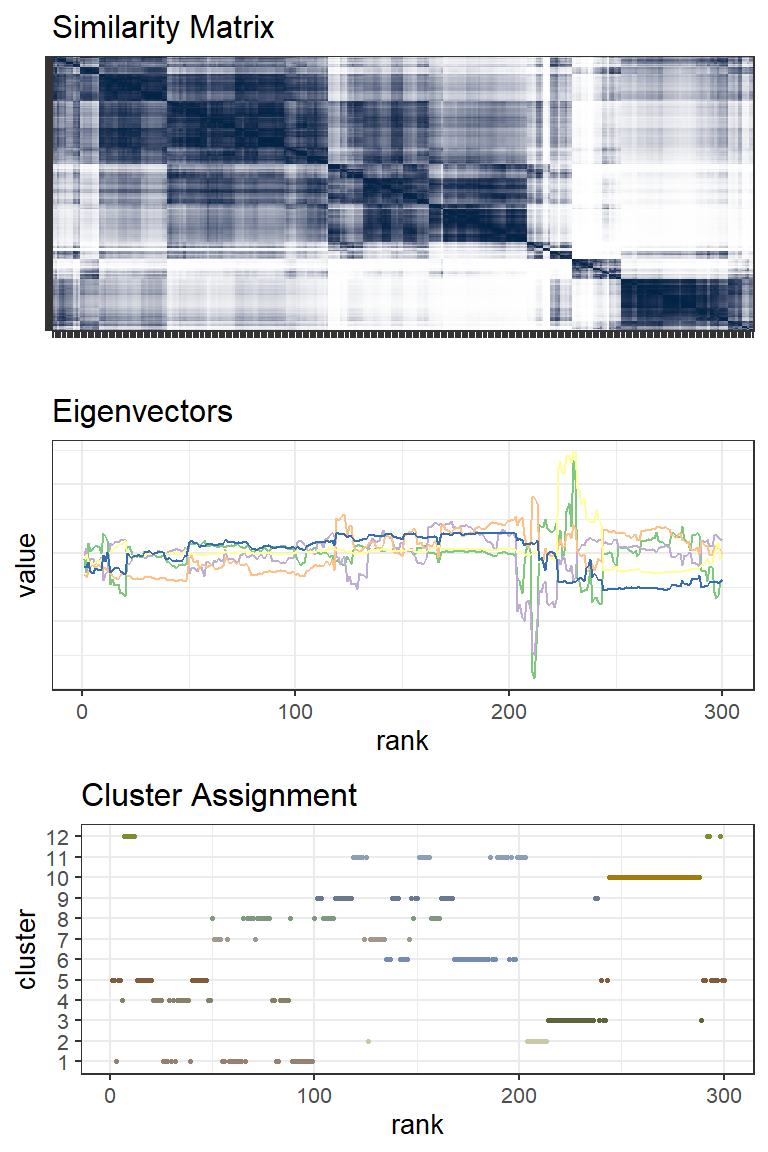
Using a Radial Basis Function (RBF) kernel the data are converted to a similarity matrix. The kernel inserts non-linearity into the analysis allowing us to find complicated boundaries between clusters. And it’s controlled by a single parameter, sigma, the variance of the Gaussian distribution. The similarity matrix is visualized below (after some re-ordering) for the same 300 points. Clusters are more distinct now but where shall we put the boundaries? That’s where the magic of linear algebra comes in. After some matrix normalization the eigenvectors associated with the lowest non-zero eigenvalues distinguish the clusters quite well. (Actually the eigenvector for the first lowest eigenvalue doesn’t have any value for clustering but the next handfull do.) K-means clustering or similar can then be used with the eigenvectors as input.
Conclusion
The figures above highlight a series of points ranked ~240-280 that form a distinct and well defined cluster (cluster 10, brown color). Below a selection of those points are plotted: the Bed and Chair from the painting.
